Machine learning: we briefly present some models for the integration of machine learning for the study of time series.
Machine Learning has become very popular in recent years, thanks to the growth in computing power and the ability to parallelize operations offered by tools such as GPUs and various derivatives (for example, TPUs).
This article is a continuation of the series that began with Time Series Analysis, Part 1.
Machine Learning and Time Series
Predicting the future development of a time series can be a rather complicated and inaccurate task, especially in those areas where the phenomenon recorded in the time series is subject to random fluctuations or whose causes are unknown and difficult to analyze. Recently, however, the use of Machine Learning methods in time series forecasting has yielded interesting results, especially with regard to short-term forecasting. We present in the next section a class of Machine Learning models: recurrent neural networks.
Neural Network and Time Series
Neural networks have demonstrated good results in applications in various fields. One of these is the prediction of future values of a time series.
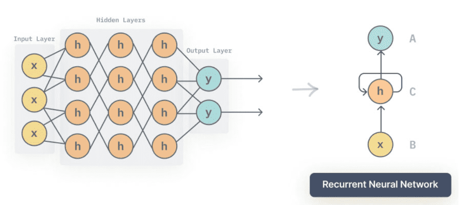
The simplest neural network model is a feedforward, fully connected neural network. This means that the neural network processes data in only one direction, from input to output, without feedback; moreover, each unit (also called a “neuron”) in each layer is connected to each unit in the next (and previous) layer.

In the example in the previous image we see a neural network formed by the input layer (in purple), two hidden layers (those formed by the units in green) and an output layer. In this example we are dealing with a classification problem: the model receives four values as input and produces three values as output, which somehow represent the expected class of the input.
Such a type of neural network is not suitable for use in the field of time series: this is due to the fact that the neural network receives all inputs at a given (initial) time, so it is not able to analyze the properties of a sequence.
A more suitable architecture for time series analysis is that provided by recurrent neural networks, for which the state of the network at a certain point in processing can affect subsequent processing.

In the figure above we see how, in a recurrent neural network, there is some kind of self-action, self-feedback of the units “on themselves”: this feature allows recurrent neural networks to be adapted to time series analysis.
Recurrent neural networks, however, have some problems related to training difficulty, particularly the vanishing/exploding gradient problem. We do not want to go into the presentation of this problem here, suffice it to say that there are neural network models that make it possible to avoid this drawback: the Long-Short Term Memory network (LSTM) e i Gated Recurrent Unit (GRU).
From a practical point of view, it is very simple to set up a neural network that, given n steps in a time series, predicts the value at the next time. To do this, we need to set up the network’s training data sequence so that the problem can be transformed into supervised learning. Suppose our time series is given by the sequence of data:
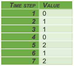
Suppose further that we want to train our network to predict the next value from the sequence of the previous three values. We then set up a table where we associate each data item with the sequence of the previous three data items:

We then divide our data into two parts: the test data, X_test and y_test, and the training data, X_train and y_train. We ignore the validation problem for the moment, imagining that we are using fixed hyperparameters (the number of units, the optimizer, the loss function, …). Also, let us imagine that we have already normalized the data (e.g., using a sklearn.preprocessing.MinMaxScaler.
We define an LSTM network using keras:
lstm = Sequential()
lstm.add(
LSTM(
50,
return_sequences=False)
)
lstm.add(Dense(1))
We then proceed to the compile phase:
lstm.compile(
optimizer=”adam”,
loss=”mean_squared_error”,
metrics=[“accuracy”]
)
Finally, we perform the network fit:
lstm.fit(
X_train,
y_train,
batch_size=1,
epochs=10
)
lstm.summary()
At this point, we can use the network to make predictions about the test data and evaluate performance:
y_hat = lstm.predict(X_test)
A similar network could produce predictions like those in the following image:

It should be remembered that the network predicts only the next value for each step sequence: it is a case of single-step prediction.
A concrete example: we may want to predict the value of a stock given the history of values in the previous three days. This model does not allow us to make long-term predictions, but it can be very useful for short-term trading.
Another example, coming from the industrial world, could be the prediction of an (average) temperature measurement for a subsequent unit of time (say an hour) based on the temperatures of the previous three hours.
Multi-Step Prevision
Predicting multiple time steps is a more complex problem. The neural network must attempt to extrapolate a model that represents the dynamics of some step of the phenomenon, which, in some cases, turns out to be really complicated. Often, such multi-step forecasts have error rates that rather increase as the steps progress: the next-day error is likely to be smaller than the one-day error n+2.
Conclusions
In this article we presented some ideas of how neural networks can be used to study and predict the future behavior of time series.
There is no need to underline that here we have limited ourselves to the essential concepts; the techniques used in real projects are nowadays much more complex and require familiarity with more complex algorithms than those mentioned here.
