Introduction
Convolutional Neural Networks (CNNs) have transformed the field of computer vision, making it possible to successfully tackle complex tasks of image processing and interpretation. Among the most significant architectures, ResNet (Residual Network) stands out for its ability to efficiently manage deep networks. Introduced by Kaiming He in 2015, ResNet has had a remarkable impact in the field thanks to its innovative structure based on residual connections, which simplify the flow of information within the network.
Use of Pretrained Models
Transfer Learning
One of the most common approaches when working with complex architectures and limited dataset resources is transfer learning. This approach involves using a model pre-trained on a large dataset and then adapting it to a new task. ResNet50, due to its ability to capture complex features of images, is particularly suited for transfer learning.
The concept of fine-tuning involves reusing the weights of a pre-trained model and adapting its final layers to the new problem. This approach significantly reduces training time, especially when data available for the new task is limited.
For fine-tuning ResNet50, most of the pre-trained layers are frozen (so they are not updated during training), and only the final layers or new additions, such as a classification layer specific to the new dataset, are trained.
ResNet Architecture – Overview
ResNet introduces the concept of residual learning, which facilitates the training of very deep networks. The main idea is the use of skip connections(#skip-connections-an-in-Depth-look), which bypass one or more convolutional layers and add the output directly to a later layer. This structure helps preserve gradients during backpropagation, mitigating the vanishing gradient problem see more below(#the-vanishing-gradient-problem).
Residual Blocks
The core of ResNet is the residual block, which can be represented as:
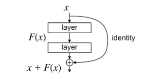
![\[y = F(x) + x\]](https://www.aiknow.io/wpvt/wp-content/ql-cache/quicklatex.com-aeed31f4311fef3a9e2d0a85ff4f3465_l3.png "Rendered by QuickLaTeX.com")
where  is the input,
  represents a nonlinear transformation applied by a series of convolutional layers, and
  is the final output of the block. This direct connection between input and output helps the network retain crucial information and accelerates convergence during training.
is the input, represents a nonlinear transformation applied by a series of convolutional layers, and is the final output of the block. This direct connection between input and output helps the network retain crucial information and accelerates convergence during training.
Skip Connections: An In-Depth Look
Skip connections are one of the key aspects that make ResNet particularly powerful. In a traditional neural network model, information passes through all the layers of the network, with no possibility of “skipping” intermediate layers. However, in ResNet, **skip connections** allow part of the information to bypass one or more convolutional layers and be added directly
to the final result of a deeper layer.
Skip connections are useful for two main reasons:
- Improvement of gradient flow: In deep neural networks, the gradient can decay exponentially as it is backpropagated, especially in the early layers of the network. This phenomenon is known as the vanishing gradient problem. Skip connections allow gradients to pass directly through the layers without significant attenuation, thereby improving learning in very deep networks.
- Facilitation of training: Skip connections help the network focus on high-level tasks and not have to memorize less relevant details, promoting better generalization. Without these connections, very deep networks might suffer from a “learning saturation” effect, where weights tend to not change or converge too slowly.
ResNet: Architecture and Functioning
1. Structure of Residual Blocks
A ResNet block is composed of several convolutional layers, followed by normalization and activation functions.
The basic structure of a ResNet block includes:
- 3×3 Convolution (
 ): captures local spatial features.
 - Batch Normalization (BN): normalizes the output to improve training stability.
- ReLU (Rectified Linear Unit): introduces non-linearity.
- Sum with the original input (skip connection): allows direct flow of information.
The mathematical operation of a residual block can be expressed as:
where:
- is the input to the block,
- represents the nonlinear transformation applied by the set of operations (Conv, BN, ReLU),
- is the output of the block, which sums _F(x)_ with the original input.
More specifically, can be expressed as:
can be expressed as:
![\[F(x) = W_2 \sigma(W_1 x)\]](https://www.aiknow.io/wpvt/wp-content/ql-cache/quicklatex.com-d2418c374d25806bb9a6631837eaff90_l3.png "Rendered by QuickLaTeX.com")
where:
 and
and  are the weights of the convolutional layers,
 is the ReLU activation function.
If the dimensions of the input and output do not match, a linear transformation is used through a  convolution:
convolution:
![\[y = F(x) + W_s x\]](https://www.aiknow.io/wpvt/wp-content/ql-cache/quicklatex.com-680ff37c3d7aa207e3b2322fdb75df24_l3.png "Rendered by QuickLaTeX.com")
where  is a transformation matrix.
is a transformation matrix.
2. Life Cycle of ResNet
The life cycle of the ResNet architecture involves several phases:
2.1. Model Preparation
-
-
- Definition of the architecture (number of residual blocks, filter sizes, etc.).
- Initialization of the weights.
-
2.2. Training
-
- Forward pass: propagation of the input through the network.
- Calculation of the loss function.
- Backpropagation: updating the weights using the gradient descent algorithm (SGD or Adam).
- Use of skip connections to improve gradient flow.
2.3. Validation and Testing
-
- Evaluation of performance on unseen data.
- Possible fine-tuning or adjustment of hyperparameters.
2.4. Inference
-
- Use of the trained model to make predictions on new data.
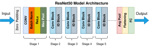
3. ResNet-50: Specific Structure
ResNet-50 is a specific version of ResNet with 50 layers, organized as follows:
- A first convolutional layer (
 , stride 2)
 - A max-pooling layer (
 )
) - 4 residual blocks with (3, 4, 6, 3) sub-blocks each
- A final fully connected layer for classification
The depth of the network allows it to capture advanced hierarchical features, making ResNet-50 effective for complex computer vision tasks.
ResNet50 is one of the most widely used variants because it offers a good balance between depth and computational efficiency.
Its architecture consists of:
- An initial convolutional layer followed by max-pooling.
- 16 bottleneck blocks organized into four groups.
- An average pooling layer and a final fully connected layer.
Bottleneck Blocks
Unlike standard residual blocks, *bottleneck blocks* use a sequence of three convolutions with kernels of size (1×1, 3×3, 1×1):
- 1×1 Conv – Reduces dimensionality.
- 3×3 Conv – Processes features.
- 1×1 Conv – Restores dimensionality.
This configuration helps keep the number of parameters manageable even in deep architectures.
Advantages of ResNet and ResNet50
- Mitigation of vanishing gradient: Thanks to skip connections, gradients can flow without degrading.
- Greater depth without increasing computational complexity: Bottleneck blocks improve efficiency compared to standard residual blocks.
- High performance on ImageNet and other datasets: ResNet50 is widely used for classification, segmentation, and object recognition.
- Transfer learning: ResNet50 pre-trained on ImageNet is often used for fine-tuning in various applications.
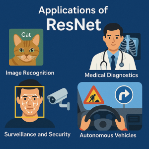
Applications of ResNet50
ResNet50 is used in various contexts, including:
- Image Recognition: Object classification in datasets like ImageNet.
- Medical Diagnostics: Identification of diseases from medical images.
- Surveillance and Security: Facial recognition and video analysis.
- Autonomous Vehicles: Identification of road signs and obstacles.
Problems and Limitations of ResNet
Computational Complexity:
Despite the significant advantages offered by ResNet50, such as reducing the risk of vanishing gradient with skip connections, it is still a very deep and complex model. Its depth implies a considerable amount of computational operations. This can be a challenge on devices with limited resources, such as mobile or embedded devices. Inference times can be slow, and high memory usage can be problematic for applications requiring a fast response.
Overfitting with Limited Data:
Although ResNet’s skip connections improve learning ability and generalization, the model can still suffer from overfitting when the available data is limited. This is especially true if the dataset is not diverse or representative enough. In these cases, the deep architecture might “memorize” the training data instead of generalizing.
An effective solution to counteract overfitting is data augmentation, which increases the variety of the training data by modifying the images (e.g., through rotations, zooms, translations). This approach improves the robustness of the model without needing to collect new data.
Conclusion
ResNet and its variants, particularly ResNet50, have revolutionized the field of computer vision. Thanks to their innovative architecture with residual connections, these networks enable the training of deep models without encountering the typical problems of traditional CNNs. Their efficiency and accuracy make them fundamental tools for a wide range of applications.
